How to: Apply Per-Row Conditional Formatting across rows in Excel 2013

I really appreciate conditional formatting in Excel. It’s a great way to highlight critical pieces of information, provide quick visual distinctions, etc.

However, I was often confused about how to apply per-row conditional formatting to the whole table. This seemed really annoying, and so conditional formatting seemed less than useful.

Turns out, it was really easy! Which probably everyone else already knew

Below, I demonstrate two different techniques – with animations to help guide things along.

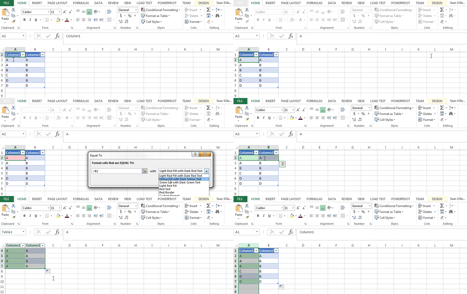
Method 1: Drag the Formatting

• Select the cell and apply the conditional formatting, referencing other cells in the row.
• Highlight the row
• Drag the corner of the row down to the bottom of the cells you want to apply the formatting to – just as if you were going to replace all the content.
• However, an icon appears in the lower-right-hand corner. Click this icon
• Select “formatting only” to replace the formatting only, which will include the conditional formatting.

Example below (click to expand):

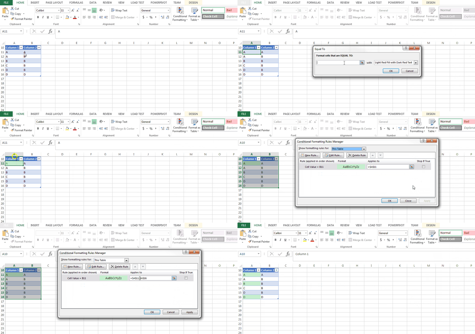
Method 2: Edit the Rule Manually

• Select the cell and apply the conditional formatting, referencing other cells in the row.
• Highlight the table or group of rows
• On the conditional formatting menu, select Manage rules...
• Edit the cell list that the rule applies to.

Excel will automatically recalculate the references and you’ll be on your way!

Example below (click to expand):

Hope this helps! Let me know if you have any questions (or a better method!) in the comments.