Excel Tip: Generate a Defined Name from a Table

Sometimes you may have a need to treat a column of data in an Excel table as a list – for example, to use the contents of that list as a drop-down somewhere else.

To do this, you’ll first have to create a named range for the table, which isn’t done the way it is elsewhere.

To demonstrate this, I’ll use a table with some names and demonstrate the drop-down list.

Step 1: Create the table

We start off with a list of names, unformatted in Excel:

• Highlight the cells in Excel:

• And then format them as a table:

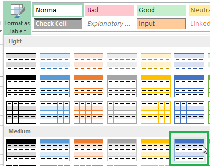
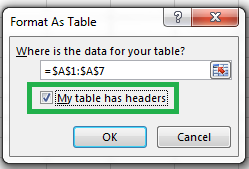
Note: Select “My table has headers” for the appropriate affect:

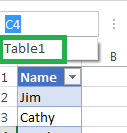
Also Note: Excel has automatically given this table a name of Table1:

Step 2: Create the Defined Name

• Head to Formulas and select Define Name:

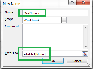
• Give the data name (in this case, OurNames).
• Set the Refers to to be =Table1[Name]. This tells Excel to set this defined name equal to the Table1 “Name” column. When you’re done, it will look similar to the below:

• Click OK. Voila, you have a defined name range!
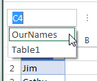
• You can verify your named range by going to the names drop-down in the top left corner, where you’ll now see OurNames. Try selecting it!

The Nice Thing About This Technique – Adding new people rows includes them!

Unlike a normal defined name, which includes a set amount of cells, a defined range based on a table includes any of the cells defined by that table – even if they were outside of the original range.

To demonstrate this:

• Add an item in the table below your last cell, e.g. “New Person”
• The table will automatically expand to include that cell
• Drop down the defined name and select it. Note that the new cell is included as well!

This is particularly useful for doing things like pulling drop-down list items from a table.